Estimating Hitting Times Locally at Scale
How to measure the distance between two nodes in a massive graph without ever seeing the whole map.
⚡ TL;DR
Problem: Calculating "Hitting Time" (distance) exactly takes $O(n^3)$ time, which is impossible for massive social networks.
Old answer: Global matrix inversions that require loading the entire graph into memory.
New answer: A local algorithm that runs two independent random walks from start and end points until they meet.
Key Insight: The "Meeting Time Identity": The infinite sum defining hitting time collapses exactly when the two walkers collide.
1 The Story in Plain English
Imagine you want to know how "close" two people are in a social network. One way to measure this is to ask: "If I start a rumor with Alice, how long until it reaches Bob?" This is called the Hitting Time.
In a small group, you can just simulate it or calculate it exactly. But in a network with billions of users (like Facebook or Twitter), calculating this exactly is impossibly slow. You'd need to know the entire structure of the network to solve the equations.
💡 The Analogy: Lost Friends
Imagine Alice and Bob are lost in a massive, foggy city. They want to know how far apart they are.
The Old Way: Alice walks randomly until she finds Bob. If the city is huge, she might wander for years in the wrong direction.
The New Way (Meeting Time): Alice and Bob both start walking randomly. Because they are both moving, they cover more ground. If they are in the same "neighborhood" (cluster), they will bump into each other (meet) relatively quickly. The time it takes them to meet is a much more stable and local measure of their proximity than waiting for one to find the other's fixed starting point.
Before We Dive In: What You'll Need
- Random Walk: A path where each step is chosen randomly from neighbors.
- Markov Chain: A mathematical system that undergoes transitions from one state to another.
- Hitting Time: The expected number of steps to reach a target node.
- Mixing Time: How long it takes for a random walk to become truly random (forget its start).
2 The Problem: The $O(n^3)$ Barrier
Formally, the hitting time $H(u, v)$ is the expected number of steps for a random walk starting at $u$ to first visit $v$.
The standard way to compute this involves solving a system of linear equations involving the graph's Laplacian matrix. For a graph with $n$ nodes, this takes roughly $O(n^3)$ time (matrix inversion).
🤨 Reality Check
Q: "Can't we just run a simulation?"
A: You can, but the variance is huge. A random walk might get "lost" in a distant part of the graph and take millions of steps to return, even if the target was just one hop away in the other direction. Naive Monte Carlo is too slow.
Interactive: The Meeting Game
Click "Start" to release two random walkers (Blue and Red). Watch how quickly they find each other compared to exploring the whole grid.
3 The Key Insight: Meeting Times
The authors prove a remarkable identity that connects the global Hitting Time to the local Meeting Time.
Instead of simulating one walker from $u$ to $v$ (which might wander off forever), we simulate two walkers: one starting at $u$ ($X_t$) and one starting at $v$ ($Y_t$).
We stop the simulation as soon as they meet (at time $T$). The paper shows that we can estimate the hitting time using only the path history up to this meeting point.
Math Deep Dive: Lemma 4.1 (The Identity)
The core estimator is based on this identity:
Where:
- $T$ is the meeting time (when $X_t = Y_t$).
- $\mathbb{I}_{[Y_t=v]}$ counts if the walker from $v$ is at $v$.
- $\mathbb{I}_{[X_t=v]}$ counts if the walker from $u$ is at $v$.
Translation:
"Run two walkers until they meet. Count how many times the walker starting at $v$ loops back to $v$, and subtract how many times the walker starting at $u$ accidentally hits $v$ before meeting. The average of this difference is the Hitting Time."
Math Deep Dive: Meeting Time Bound
Why is this efficient? Because walkers meet quickly in local neighborhoods. The probability that they haven't met by time $t$ drops exponentially:
Deconstructing the Terms
- \(\pi_G(u), \pi_G(v)\): The stationary distribution probabilities of the start nodes. If $u$ and $v$ are "important" (high degree) nodes, $\pi$ is larger, making the initial factor smaller.
- \(t_{\text{mix}}\): The Mixing Time of the graph. This is the time it takes for a random walk to become truly random. A smaller mixing time means faster convergence.
- \(\|\pi_G\|_2^2\): The collision probability of the stationary distribution. It measures how "concentrated" the graph is.
Takeaway: Unless the graph is extremely "slow" (high $t_{\text{mix}}$), the walkers are guaranteed to meet quickly, meaning we don't need to simulate for long.
Main Contributions
1. Meeting Time Algorithm
We design and analyze an efficient local algorithm (Algorithm 1) based on the novel analysis of meeting times. It's unbiased and practical for massive graphs.
2. Spectral Cutoff Extension
We extend the work of Peng et al. [2021] to derive Algorithm 3. It uses spectral decomposition to truncate the hitting time sum. While generally slower than meeting times, it can be better in specific settings.
3. Theoretical Trade-offs
We provide a detailed study of the trade-off between approximation error and sample complexity, proving both upper and lower bounds (Section 5).
4. Property Testing Link
We uncover a connection to sublinear-time property testing. Finding the "local mixing time" is analogous to testing if a distribution is close to uniform, allowing for sublinear algorithms.
The Algorithms
Algorithm 1: Meeting Time Estimator
This is the core contribution. It estimates $H(u,v)$ by running paired random walks.
- Initialize sum $Z = 0$.
- Start random walk $X$ at $u$ and $Y$ at $v$.
- Repeat until $X_t = Y_t$ (Meeting Time $T$):
- If $Y_t == v$, add 1 to $Z$.
- If $X_t == v$, subtract 1 from $Z$.
- Step both walkers.
- Return $Z$. (Average over multiple runs for accuracy).
Algorithm 3: Spectral Cutoff
While Algorithm 1 uses random walks (Monte Carlo), Algorithm 3 takes a linear algebra approach.
The Idea
The hitting time can be expressed as a sum of the graph's eigenvalues and eigenvectors. $$ H(u,v) \approx \sum_{k=1}^{N} \frac{1}{1-\lambda_k} (\dots) $$
The "Cutoff" Trick
Terms with small eigenvalues ($\lambda_k \approx 0$) decay very fast. We don't need to sum them all! Algorithm 3 only computes the first few "slowest" modes (largest $\lambda_k$) and ignores the rest.
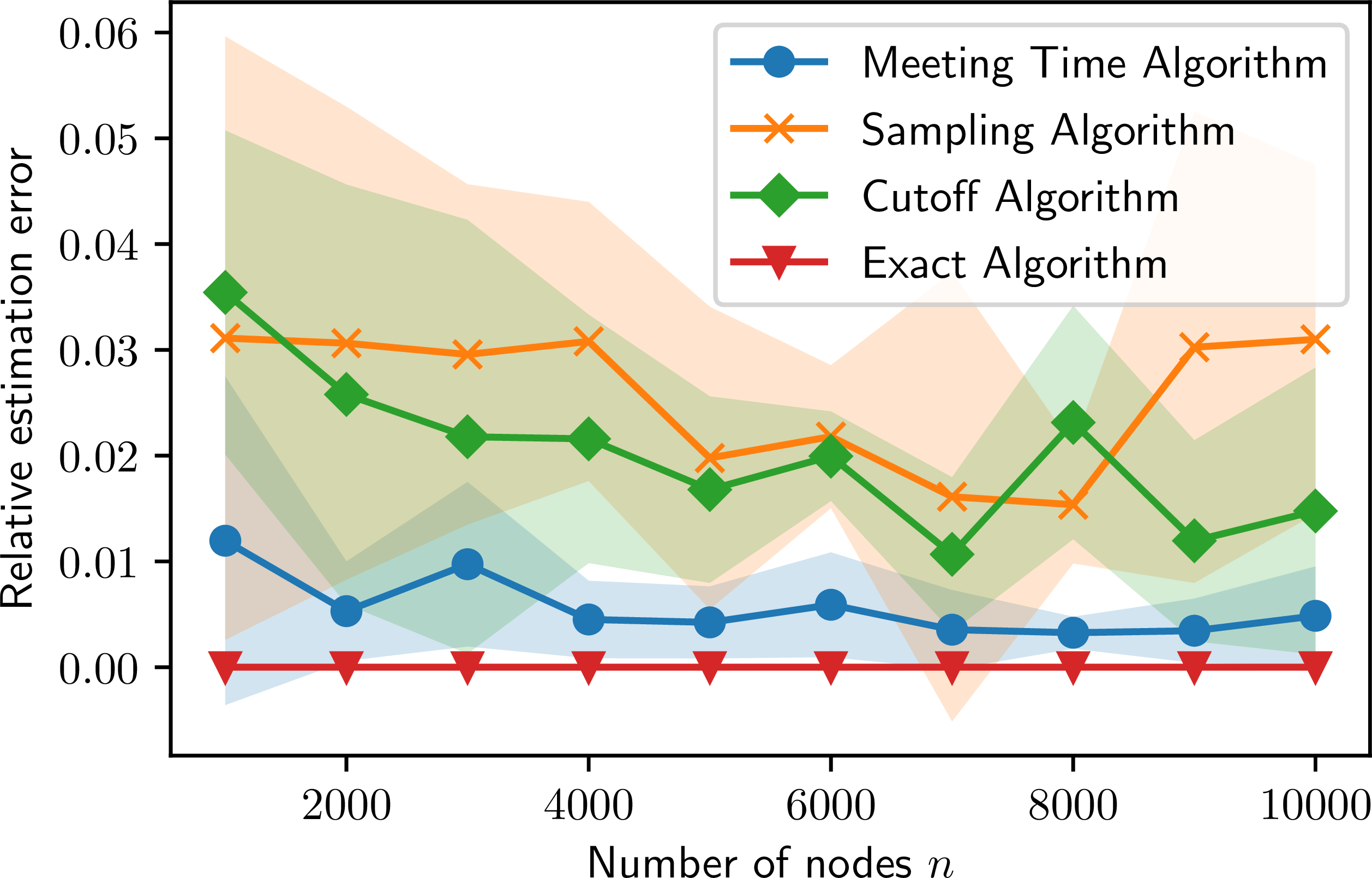
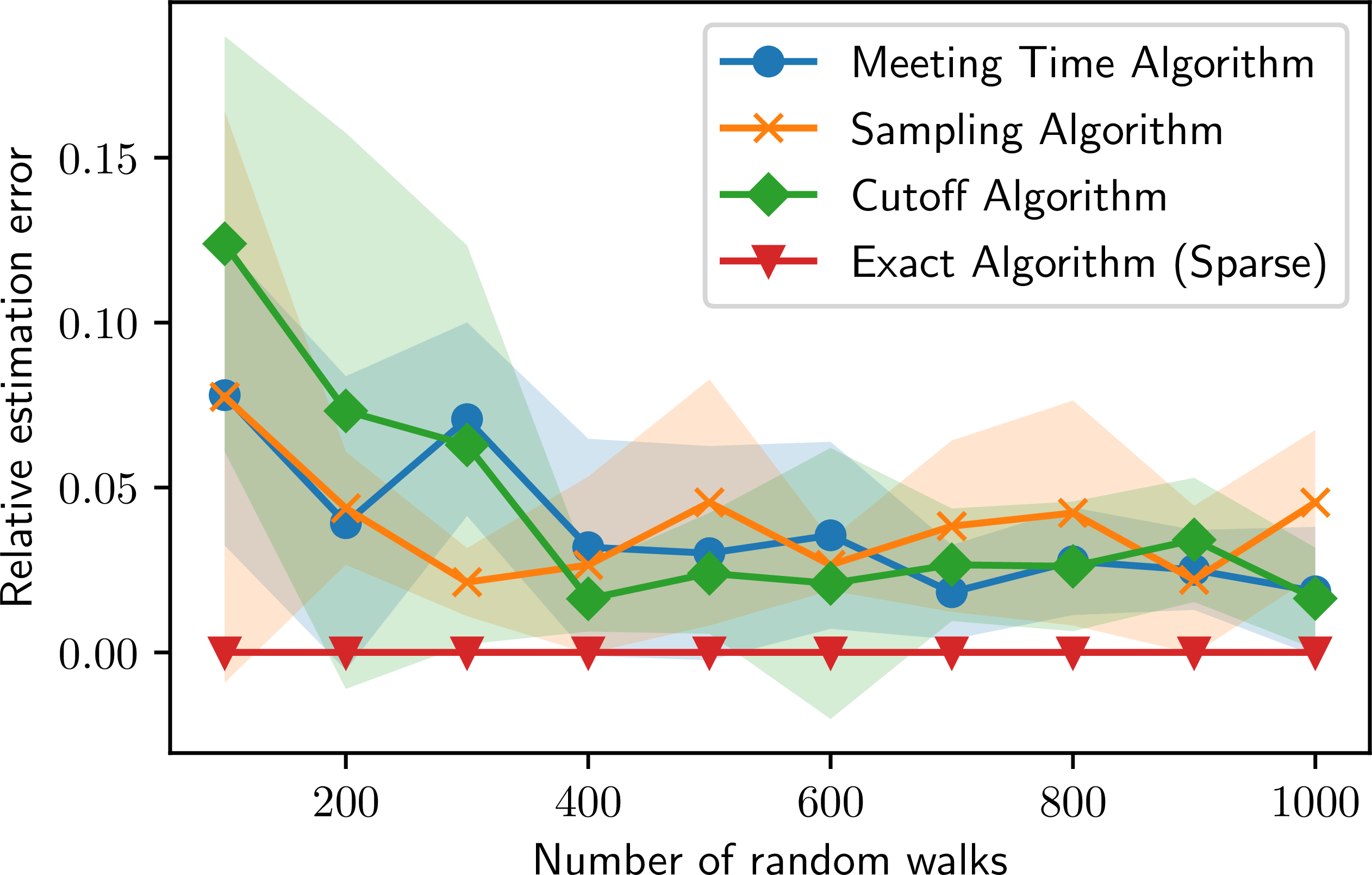
Experimental Results
The authors rigorously tested their algorithms on both controlled synthetic environments and messy real-world social networks.
Synthetic Benchmarks
They used Erdős-Rényi (random), Barabási-Albert (scale-free), and Stochastic Block Models (communities) to test scalability.
Key Finding: The Meeting Time algorithm maintains low error and low variance even as the graph size ($n$) grows, whereas naive sampling struggles.
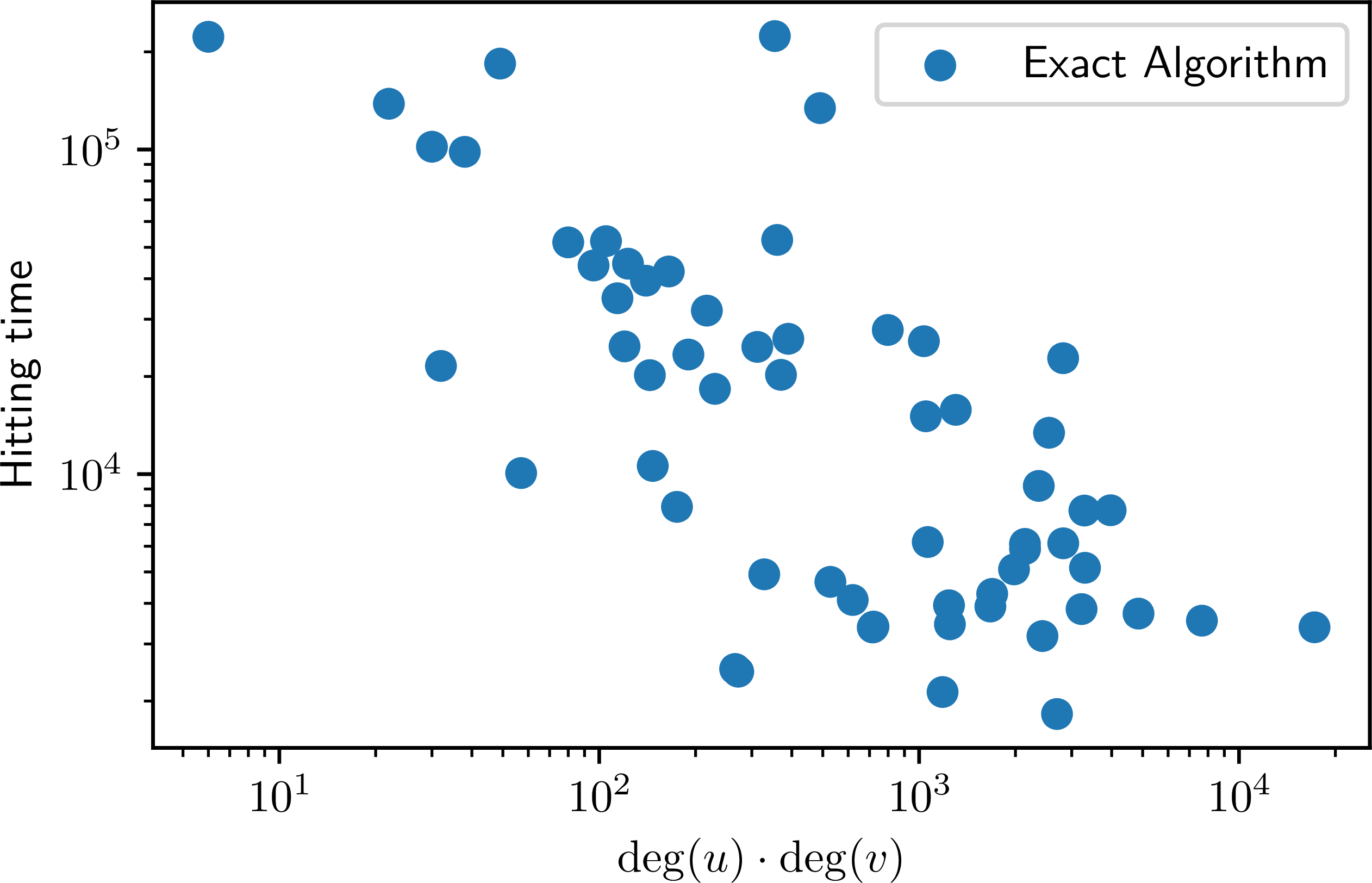
Real-World Stress Tests
Tested on SNAP Facebook (social circles) and Twitter (massive follower graph). They sampled pairs of users in three ways: uniformly, high-influence (hubs), and low-influence (peripheral).
Key Finding: The algorithm achieved ~1% relative error consistently across all types of user pairs, proving it works for both "celebrities" and "regular users."
🧐 Critical Analysis: Strengths, Weaknesses & Open Questions
✅ What This Paper Does Well
- Truly Local: It doesn't need to touch the whole graph. This is a game-changer for billion-node graphs.
- Unbiased: Unlike some heuristics, this estimator converges to the exact true value.
- Simple: The core algorithm is just "run walks until they meet".
⚠️ Legitimate Concerns
- Mixing Time Dependency: If the graph has "bottlenecks" (bad mixing time), the walkers might take a long time to meet, slowing down the algorithm.
- Variance: While unbiased, the variance can still be high for certain graph topologies, requiring many samples.
🎯 Bottom Line
A clever and rigorous application of probability theory that solves a real scalability bottleneck. It turns a global matrix problem into a local simulation problem.